
Overview of the Graphics Pipeline
This post will talk about basic concepts of computer graphics. More specifically it will go over the entire graphics pipeline in a conceptual (high) level. It will go into detail on each stage of the pipeline to give the reader a high level view of the process that is required for any kind of real-time graphics to appear on the screen. This post serves as a basis for future posts that will use the terminologies and concepts of the graphics pipeline.
The Graphics Rendering Pipeline
The graphics rendering pipeline is the most important concept in real time graphics. For geometry to be displayed to the screen it must go through each stage of the graphics pipeline. In the physical world, a pipeline consists of a series of stages each responsible for a specific task. Take for example a factory assembly line. Each stage of the assembly line executes a specific task and the full product is complete after it exits the last stage of the pipeline. Pipelines operate in a first in first out fashion. Elements entering the first stage of a pipeline cannot move to the second stage until the elements already processed by the second stage move to the third and so on and so forth. Like the pipelines in the physical world, the graphics rendering pipeline processes geometry through various stages until this geometry exits the pipeline in the form of a pixel ready to be output to the screen of the device.
Pipelines are a highly parallelizable construct. Each stage of the pipeline can run in parallel and is only delayed until the slowest stage has finished its processing. So, in a system that does not use a pipeline, adding a pipeline of n stages, could result in a speedup of a factor of n.
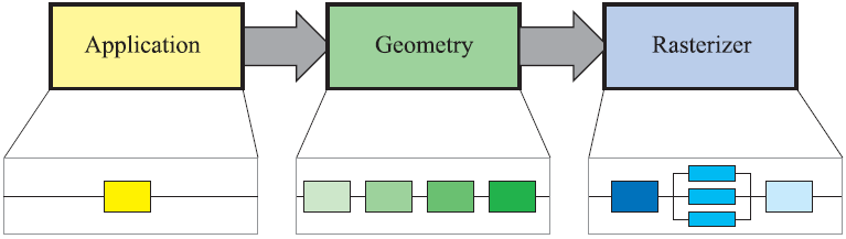
As in the image above, the graphics rendering pipeline can be divided into three conceptual categories, the application stage, the geometry stage and the rasterizer stage. Each one of these three conceptual stages can be implemented as a pipeline itself containing functional stages and each functional stage can be divided into pipeline stages. Functional stages perform certain tasks but do not define the way they are executed in the pipeline. Pipeline stages are executed in parallel with other pipeline stages and can also be parallelized. How the task of a functional stage is executed depends on the implementation, for example the geometry stage can be divided into five functional stages, but the implementation decides how many pipeline stages will exist in each of the functional stages and how many of them will run in parallel.
The Application Stage
The application stage is controlled by the application which means it is controlled by software running on general purpose CPUs. These CPUs include multiple cores and can utilize multiple threads of execution in parallel to execute many various tasks that may be needed by the application like preparing the geometry data before submission to the GPU for rendering, physics simulation, animation, AI and many more. The application stage is under the full control of the developer, granting the opportunity to determine the implementation and, allows for design revisions if needed to improve performance. Changes made here can have an impact on the later stages of the pipeline. For example, if the application manages memory allocation logic poorly, the geometry stage’s performance will suffer. In the context of a graphics application, the application stage’s most important task is to prepare and submit the geometry to the geometry stage for rendering. The geometry prepared and submitted to the geometry stage consists of rendering primitives like points, lines and triangles that might end up being displayed on the screen.
The Geometry Stage
The geometry stage’s main responsibilities are per-polygon and per-vertex operations and can be divided to the following functional stages: model and view transformation, vertex shading, projection, clipping and screen mapping as depicted in the image bellow.
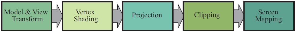
Depending on the implementation these functional stages may or may not correspond to actual pipeline stages since some implementations may merge functional stages together to form a single pipeline stage or further divide them to multiple pipeline stages.
Model and View Transformation
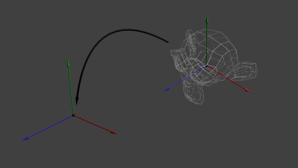
Before geometry reaches the stage of being displayed on the screen, it gets transformed into several different coordinate systems also known as coordinate spaces. When geometry is first defined, it resides in a coordinate space called local or model space. The local space is a coordinate system that is defined relevant to an arbitrary origin chosen by the artist designing the geometry, or the application if it is generated procedurally and serves the purpose of providing convenience during the definition of the geometry. If geometry is in local space it means that it has not been transformed at all and all the vertices are defined relative to the origin of the local coordinate system which is usually the center of the 3D model. For geometry to be positioned and oriented within the three-dimensional world it must be transformed from the local/model coordinate system to the world coordinate system or world space. In world space, the vertices go from being defined relative to the origin of the model, to being defined relative to the origin of the world. Each model (group of geometry) can be associated with a model transform and thus allowing for same geometry to be placed multiple times within the world without the need to duplicate its data. The process above is illustrated in image bellow.
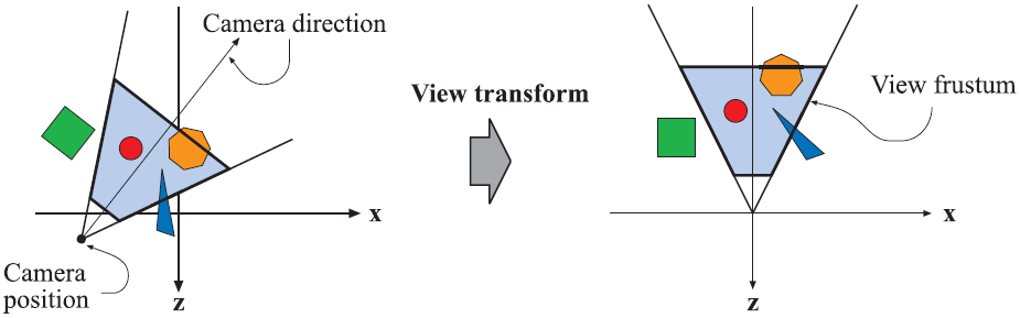
After all the models have been transformed by their associated model transform, they all reside in this same space. For the geometry to appear on the screen it must be in view. The view is just a transformation in computer graphics but, to make it easier to understand, developers created an abstraction on top of it called the camera. The camera has a position in the world and a direction. After the camera has been placed and oriented in world space along with the rest of the geometry, the view transform is applied. The view transform’s purpose is to place the camera in the origin of the world coordinate system and aim its direction down the positive or negative z-axis (depending on the implementation), aligning the geometry in the same way as well as shown in image bellow. This allows the projection and clipping operations that follow down the pipeline be simpler and faster.
After the view transformation is applied, the new coordinate system is known as the view coordinate system or view space. The model and view transformations along with any other form of coordinate system transformation that occurs within the pipeline are applied using 4x4 mathematical matrices, the main reason being their ability to concatenate and store information about multiple transformations.
Vertex Shading
The vertex shading stage is where the main vertex processing occurs. At this stage vertices are processed and transformed to the correct coordinate space to be shaded. Shading is the operation performed to determine the effect of a light source on the geometry. To accomplish that, the shading equation is evaluated at various points on the object to calculate the amount of light received at each one of these points. The amount of light received in combination with the object’s material determine the appearance of the object after the shading operation is concluded. Materials are a description of an object’s appearance in the world. This description can be as simple as a color value or a complex physical representation of the object. The shading operation is typically performed on geometry transformed to the world coordinate system, but on many occasions, it is more convenient to perform shading in other coordinate spaces like the view space or tangent space depending on the shading effect that must be accomplished. This is possible because the relative relationships between geometry, lights and the camera are preserved if all exist in the same coordinate space. It is worth mentioning that shading can be performed in a per-vertex or a per-fragment basis. The stage at which shading is performed has a different impact on the object’s appearance and the computational power needed for the operation.
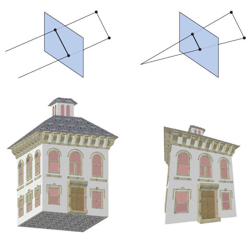
Projection
Projection is the process of transforming the view volume into a unit cube with its extreme point values being [-1, 1] in all three axes. This unit cube is known as the canonical view volume. The two most common projection methods in computer graphics are the orthographic and the perspective projection. In the case of the orthographic viewing, the view volume is a rectangular box which is then transformed into a unit cube by the projection transform. The main characteristic of orthographic projection is that lines that are parallel before the transformation remain parallel after it. The perspective projection is a more complex case. In this projection, the farther away an object is from view the smaller it appears after the transformation. In contrast to the orthographic projection, parallel lines may converge at the horizon. This change of object size with distance from the point of viewing mimics our perception of the real world when it comes to the relationship of size and distance. In geometric terminology, the view volume in perspective viewing is called a frustum and is a truncated pyramid with a rectangular base. After the perspective transformation the view frustum is transformed into a unit cube as well. Geometry that has undergone projection resides in a coordinate space known as normalized device coordinates. In summary, the projection transformations convert the geometry from three dimensions to two. The third dimension, depth, is not stored in the generated image. It is stored in a separate buffer known as the Z-buffer (also known as depth buffer) which will be discussed further in the rasterizer stage section. The image bellow shows the difference between the two projections.
Clipping
After applying the view and projection transformations, primitives that reside inside the view volume pass to the next stage of the pipeline, and primitives that reside outside the view volume do not since they are not rendered. Some of the primitives reside partially within the view volume. These primitives must undergo the process of clipping. The vertices of the part of the primitive that is outside the view volume get clipped against the unit cube and are replaced by new vertices located at the position where the geometry intersects the view volume as shown in the next image.
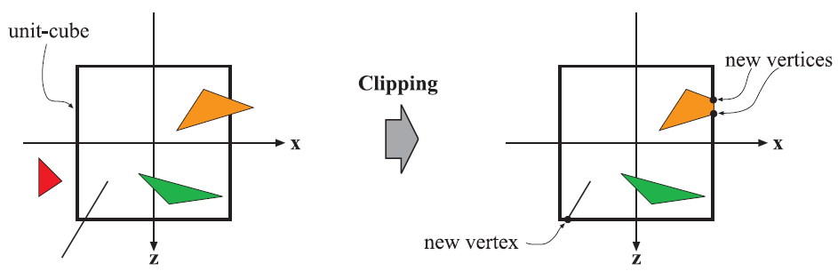
The main advantage of performing clipping after the view and projection transformation is that it simplifies the problem and makes it consistent. Primitives are always clipped against the unit cube.
Screen Mapping
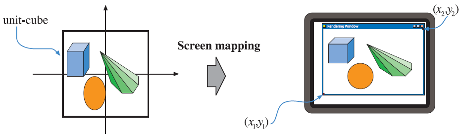
After clipping is concluded, the geometry that is in view is ready to be transformed from normalized device coordinates to screen coordinates. This operation maps the normalized device coordinates [-1, 1] to the size of the viewport. The viewport is the 2-dimensional area that the rendered image is going to occupy inside the window and usually it has the same dimensions as the window itself. This mapping is done by applying the viewport transformation, which is a scaling operation followed by a translation, on the normalized device coordinates. These new coordinates are screen coordinates and along with the z- coordinate, whose values range from [-1, 1] or [0, 1] depending on the underlying implementation, are known as window coordinates. After screen mapping is complete the data are passed to the rasterizer stage for further processing. The next image shows the screen mapping process.
The Rasterizer Stage
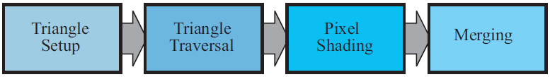
Entering the rasterizer stage, the transformed and projected vertices along with their shading data are going to be processed to compute the colors of the pixels covered by the geometry. This process is defined as rasterization or scan conversion. This conceptual stage, like the geometry stage, is divided into several functional stages. These stages are: triangle setup, triangle traversal, pixel shading and merging.
Triangle Setup
Triangle setup is the stage responsible for calculating various data about the tringle’s surface. This data is used to interpolate the shading data originating from the geometry stage as well as for scan conversion. This process, same as clipping from the geometry stage, is performed by specialized hardware on the GPU.
Triangle Traversal
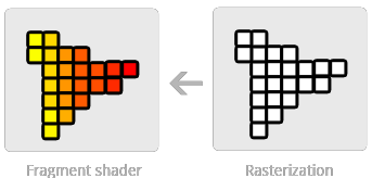
At the triangle traversal stage, it is determined which pixels have their center covered by each triangle of the geometry. A fragment is generated for the part of the pixel that is covered. Fragments are a collection of values produced by the rasterizer and represent a sample-sized part of the primitive that is rasterized. The size of the fragment is relative to the pixel area, but the rasterizer can produce multiple fragments from the same triangle per-pixel.
Each fragment possesses certain properties that are generated by the interpolation of values between the three vertices of the triangle and include the depth value and any shading data produced by the geometry stage.
Fragment Shading
The fragment shading stage is where all per-fragment computations occur. These computations use the interpolated shading data produced by the triangle traversal stage. The purpose of the fragment shading stage is to compute a final color value, considering all the shading data provided from the previous stage, for each fragment who is then submitted to the next stage. It is worth noting that there is some debate amongst developers as to if this stage is called the fragment shading stage or the pixel shading stage. In OpenGL and Vulkan nomenclature, the preferred term is fragment shading and that is because a fragment does not always correspond to one pixel. As mentioned in the triangle traversal section above, many fragments may be generated per pixel sample area depending on the state submitted from the graphics API (e.g. multisampling). Additionally, not all fragments of this stage will be displayed on the screen and become pixels since they may fail to pass certain tests on the next pipeline stage.
Merging
The merging stage is the last functional stage before pixels appear on the screen. In this stage the shaded fragments coming in from the fragment shader stage are put through a series of tests known as raster operations or blend operations. The fragments that pass this series of tests are then stored in the color buffer. The color buffer is a rectangular array of colors, each one of them consisting of a red, blue and green component. In contrast with the shading stages of the pipeline, the merging stage is not fully programmable but is highly configurable through graphics APIs, enabling different visual effects. This stage is also responsible for resolving depth visibility. Only objects visible from the point of view of the camera should be stored in the color buffer. To achieve that, the Z-buffer is used.
The Z-buffer is a separate buffer used by the GPU to store the z-coordinate (depth) values after projection occurs in the geometry stage. Before writing the color of a fragment in the color buffer, the GPU samples the value of the Z- buffer at the specific pixel location and compares it with the depth value of the fragment that is to be output on the screen. If the value already stored in the Z-buffer is smaller than the depth value of the current fragment, then the fragment is behind the fragment that is already present in the color buffer, thus it is discarded. It is worth mentioning that the way this comparison happens and the format of values inside the Z-buffer are configurable. The image bellow is a visualization of a 3D scene’s depth buffer.
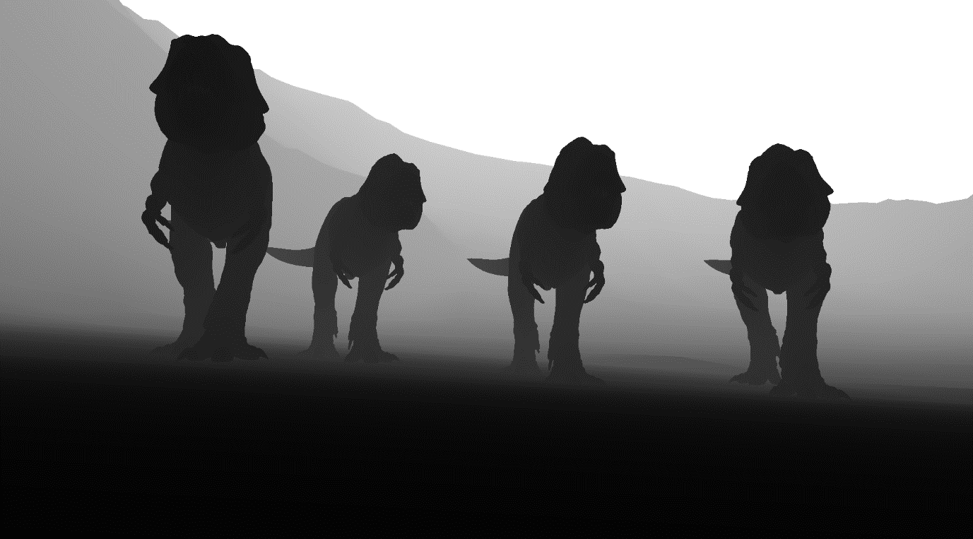
Apart from depth testing, the merging stage also deals with transparency. The color buffer apart from the red, green and blue color channels can have an extra channel called the alpha channel. This color channel represents how transparent or opaque a fragment is. The hardware uses specific blend functions to determine the final transparency value of the pixel. However, transparency is not order independent. Even though the Z-buffer allows for order independent drawing, opaque objects must be drawn before the transparent ones. This is a disadvantage of the Z-buffer algorithm. These are the main processes of the merging stage. But they are not all. Additional tests can be optionally performed like alpha testing, which using the alpha value to completely discard fragments that are bellow or above a certain threshold of transparency (alpha value), stencil testing which is performed using an additional buffer called the stencil buffer and can be used as a type of mask to what should be rendered. Finally, the accumulation buffer can be used to accumulate images using a set of operators to be used in effects like motion blur.
References
- Akenine-Möller, T., Eric, H. & Hoffman, N., 2008. The Graphics Rendering Pipeline. In: Real-Time Rendering 3rd Edition. Natick, MA, USA: A. K. Peters Ltd., pp. 12-27. Akenine-Möller, T., Haines, E. & Naty, H., 2008. Real Time Rendering. 3rd ed. Natick, MA, USA: A. K. Peters, Ltd..
- Khronos Group, 2017. Fragment.
Comments